Covid-19 Curve Model

About a month ago I was asked by a friend if it was possible to create an interactive model for Covid-19. He was having the same issue with publicity around “flattening the curve” as me.

https://www.hopkinsmedicine.org/health/conditions-and-diseases/coronavirus/coronavirus-social-distancing-and-self-quarantine

There were plenty of images like the above coming from the CDC, Johns Hokins and other institutions quickly running through media outlets. More than one world leader now has their picture taken holding printouts of the same or similar image.

While on the face its obvious what “flattening the curve” meant, the images themselves didn’t mean a whole lot. It gave us the why (why should we take this seriously) but not the when(s) and how many(s). How many beds do we have? How many people will get sick? When will the curve pass capacity? How long do we have to react?

Before looking further, let me stress: while I do have a background in Demography and statistics (with some limited epidemiology and public health experience) I am not an expert. To read more on what the experts are learning about Covid-19 I’d suggest visiting some of the usual suspects:
https://www.cdc.gov/coronavirus/2019-ncov/index.html
https://www.who.int/emergencies/diseases/novel-coronavirus-2019
https://hub.jhu.edu/novel-coronavirus-information/

Now on to my project. Last week I finished putting together a shiny app that could give some figures to the when(s) and how many(s) while allowing for different scenarios to be tested. The image below is a capture of the app’s landing page, which you can click on to open the full app in a new tab.

So what is this app? What you can see is the side panel to the left which allows user inputs. The slider allows for changes to the assumed rates associated with Covid-19, defaulting to approximate values observed in other countries with the more mature outbreaks. The numeric fields allow for changes to the at risk population. These are defaulted to the approximate values for the Country of New Zealand. As these inputs are changed, the charts to the right will display the changes to the curve.

What are the Charts?

  1. Single Day Events- the curve shows how many people will be entering the hospital, entering the ICU, or dying on a given day. For quick reference the peak curve figures are also given at the top of the chart.
  2. Cumulative Deaths- Over the span of time, the total number of people who pass from the infection.
  3. Two “Average Length of Stay Scenarios”- There is one chart for Hospitalizations and a second for ICUs. Both charts show what would happen if the average length of stay was 2, 5, or 10 days. The curves represent how many people would be in the institutions on a given day. There are also a horizontal dashed lines that represents the estimated capacities entered in the side panel.
  4. People Transitioning Between States- the number of people each day that transition from Susceptible (not infected) to Exposed (infected, not contagious); Exposed to Infected (showing symptoms and contagious); and Infected to Recovered (no longer ill or contagious).
  5. Total Population Count by Day- the Total population for a given category. Two of these are mutually exclusive, Susceptible and Recovered. It is assumed once recovered you cannot be reinfected (meaning you can never be considered Susceptible again) That is why the trade off of these two populations can be seen in the chart. The other two categories are transitional states, Exposed and Infected. These two curves show the total number of people on a given day in one of those two states.

How should I use the App? In short, however you’d like. My only hope is that between the information in this post and in the app, that the app can be informative and used responsibly. While it may be tempting to max out the rates for curiosity, please don’t snip such charts and release them into the wild without context.

Do check back in on this blog and the app, as I will likely be adding/updating content in the coming weeks.

Until then, stay well.
-Logan

Auditing Reserves and Open Space: The Value of Creating Boolean Variables

Vision recently had the privilege to work with the Far North District Council on the Reserves Audit project. Vision’s task was to create the geodatabase to serve as the foundations for future refinement and consultation.

This was one of the projects that appears simple in concept, but quickly became complex once data was collected and parameters identified. Firstly, data was coming from multiple sources in varying states of completion. This included parcel, title, and asset layers combined with ownership, ratings, DoC, and other databases. By the time all data was joined, over 50 columns were merged into a single layers datatable.

The second challenge was to figure out what needed to be extracted from the data. At the highest level, the project was about public and recreational spaces. This however broke into several subcategories depending on the type of public space of interest. Did we need to know whether the public simply had access, if it was publicly owned or managed, if the property was actually road, if the space was named, if the reserve had a designated purpose, what public assets were located on the property, if it was for conservation? The answer was “yes” to all of these and many more.

To aid in answering all of these question and combining the results, a series of boolean variables were created. Though the name may be unfamiliar, boolean variables are very commonly used and often serve as the foundation for more advanced analysis, machine learning, or AI projects. Typically they answer a logic question with one of two mutually exclusive categories (True or False, Yes or No, 0 or 1).

In total, Vision created 15 boolean variables, and an additional 2 categorical variables (similar to boolean but with multiple options). These included:

Once the required indicators were identified, the most time consuming part of the project followed: defining the criteria to calculate each indicator for parcels in the For North District. For example, we wanted to know which parcels are intended for use as road. The actual use is irrelevant; all we need to know is that there is some indication the parcel was set aside for a road propose. But, the answer to this question may be in one of 4 fields, and have several different ways of being indicated within each field.

The first stage required that Vision create summary tables of the fields for known road parcels to see what type of language or values may indicate a road. These were then entered into a selection formula, and the selected parcels reviewed to see if known parcels are missing, or if false positives exist. If known road parcels are missing, the selection formula needs refinement. If false positives exists, a second set of summaries needed to be performed to determine criteria for a de-selection formula. In the end, the criteria to select roads and deselect false positives in the Far North looked like this:

This process was performed for each of the 17 indicator variables created by Vision. With the hard part over, we were left with indicator fields that simplified the assessing open spaces in the Far North District. To demonstrate: let’s say we wanted to know every parcel that was indicated as Road or Maori purpose AND also had a Conservation or Reserve indicator. With the boolean variables, this is a relatively short expression. Without, we would have to script a convoluted selection formula.

Hopefully the comparison of formulas above highlights the benefit of using boolean variables. The time spent up front creating the indicators saves a lot more down the road. We can easily mix, match, assess, and analyse parcels across several different overlapping indicators. If we did not have these fields, we would have to script together all of the selection criteria required; each query would become long, messy, and likely impractical to the point it may not be worth trying.

In closing I should reiterate that this was the first step in the Reserve Audit work for FNDC, but the data is not perfect.  This reflects some of the issues that come with large data sets that cover many decades such as parcel and title data. Changes in recording methods, language, standards, and entry can contribute to missing or inconsistent data over time. Notwithstanding, it was a big first step that identified the bulk of public and open space in the far North, and we look forward to seeing how FNDC refines the product.  

What is NZS3604:2011 ‘good ground’?

NZS3604:2011 is the New Zealand Standard for Timber-framed buildings and is generally used to design most homes and low-rise timber framed buildings in New Zealand.  NZS3604:2011 provides standard details to meet the requirements of the New Zealand Building Code without the need for specific engineering design (SED).

For the design of foundations, the standard only applies to buildings founded on ‘good ground’. The standard defines ‘good ground’ as: “any soil or rock capable of permanently withstanding an ultimate bearing capacity of 300kPa (i.e. an allowable bearing pressure of 100kPa using a factor of safety of 3.0.), but excludes:

  1. Potentially compressible ground such as top soil, soft soils such as clay which can be moulded easily in the fingers, and uncompacted loose gravel which contains obvious voids;
  2. Expansive soils being those that have a liquid limit of more than 50 % when tested in accordance with NZS 4402 Test 2.2, and a linear shrinkage of more than 15 % when tested from the liquid limit in accordance with NZS 4402 Test 2.6; and
  3. Any ground which could foreseeably experience movement of 25 mm or greater for any reason including one or a combination of land instability, ground creep, subsidence, seasonal swelling and shrinking, frost heave, changing groundwater level, erosion, dissolution of soil in water, and effects of tree roots.

The minimum geotechnical ultimate bearing is required so that buildings are supported adequately by the ground and do not undergo differential settlement during their lifespan.  Differential settlement is when part of a building sinks more than another which can lead to uneven or cracked floors/walls.

Further, the standard states that the soil supporting the footings shall be assumed to be ‘good ground’ when all the following conditions are met:

“(a) Reasonable inquiry, through project information memorandum (PIM) and site observation show no evidence of buried services and none is revealed by excavation for footings;

(b) Reasonable inquiry, of PIM and site observation shows no indication or record of land slips or surface creep having occurred in the immediate locality;

(c) Reasonable inquiry shows no evidence of earth fill on the building site, and no fill material is revealed by the excavation for footings. This shall not apply where a certificate of suitability of earth fill for residential development has been issued in accordance with NZS 4431 for the building site, and any special limitations noted on that certificate are complied with; and

(d) Excavation for footings does not reveal buried organic topsoil, soft peat, very soft clay, soft clay, or expansive clay (see 3.2.1 and 3.3.8);

And any of the following:

(e) Where indicated by specific site investigation, using the test method for soil bearing capacity contained in 3.3;

(f) Where inspection of existing structures on this or neighbouring sites and reasonable enquiry, including territorial authority records, local history of the site, and published geological data such as structural geology where appropriate, shows no evidence of erosion (including coastal erosion, bank erosion, and sheet erosion), surface creep, land slippage, or other falling debris (including soil, rock, snow and ice), uncertified fill, fill over original water course, or subsidence having occurred in the immediate locality;

(g) When geotechnical completion reports in accordance with NZS 4404 identify subsoil class and areas that provide good ground.

If you are up for it, you can undertake an NZS 3604 Good Ground Investigation following the methods described in that document. Or keep life easy by hiring a Chartered Professional Engineer experienced in geotechnical investigations to do it for you. Don’t forget to check out the guideline for Geotechnical Investigation Requirements for Buildings in the Far North.

Completing the Elevation Model of Wellington

I’ve recently been working more in HEC-RAS and decided to have a bit of fun. Since I had already built a 3D model of  Wellington for my 3D printing project I thought, why not make some crazy flooding scenarios of the city.

However, before I could get started there was still a problem with the terrain model. The model was based off of the 1m DEM from LINZ which cut off water bodies at the water surface level. While it isn’t actually necessary have the bathymetry data for overland flooding, I wanted to have the option of dropping the waterline below sea level and also capture more realistic water depths. 

After a lot of searching I was not able to find detailed bathymetry data for the Wellington Harbour and Fitzroy Bay readily available. After contacting NIWA and they were able to provide me with a 10 meter DEM for most of Wellington Harbour and parts of Fitzroy Bay shown below. 

I merged the bathymetry data with my terrain model, and most of Wellington Harbour was complete but there were still large gaps in the channel leading into the harbour and Fitzroy Bay (lower left). Using sounding point and contour data for reference, I interpolated the missing areas in the terrain (lower right).


The animation below shows the difference between my old terrain model and the new model with the harbour bed incorporated.

I’ll note that this is a hobby project, and data is not a final or official production, but it will serve for my purposes.

Results from a preliminary flooding model are shown in the following video. Do not panic, this is the result of me throwing close to 40 meters of water at Fitzroy Bay, a rather unlikely event.

Play time aside, I’m looking forward to building multiple scenarios using project sea-rise levels and sharing those in a later post.

Predicting Subdivision With Machine Learning

At this year’s Regional ESRI Users Group conference in Whangarei, I presented Vision’s work on applying land change modelling with machine learning software to predict where future subdivisions may occur in the Bay of Islands. This is going to be a long post; so for those wanting to skip strait to the results you can have a play with the following slides. Clicking between the numbers at the top, you can see the transition between:

  1. Parcel Size (m²) in 2003,
  2. Parcel Size (m²) in 2018,
  3. Projected Parcel Size (m²) in 2038 (Inclusive Model Scenario), and
  4. Projected Parcel Size (m²) in 2038 (Exclusive Model Scenario)
[smartslider3 slider=3]

For those wanting to know more, I should first outline how this model is different from typical land change modelling. Land change models are commonly applied to changes in physical characteristics of a geographic area. This can be the land cover (eg forest converting to plains) or land use (farms land to residential). Our project is trying to measure and predict a non-physical attribute, legal boundaries. More Specifically, the transition of larger parcel size to smaller parcels. Our study area covers the Bay of Islands change from 2003 to 2018, and project the new subdivisions out to 2038.

We used machine learning software, developed by Clark Labs, to perform the raster analysis.  The process has four primary stages:

  1. Data Preparation
  2. Measuring change
  3. Modelling Susceptibility
  4. Predictive Modelling

Stage 1. Data Preparation

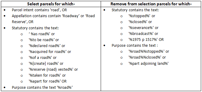
I won’t spend much time reliving this stage, partially because its boring, mostly because it turned out to be an arduous process that took about 50% of the time dedicated to the project.  What to know:

  • All data was converted to a raster format;
  • To work in the software, all data was converted to share the same CRS, extent, and grid size;
  • This project analyzed subdivision or primary parcels (not land titles);
  • Only parcels which were privately owned were retained for the model; and
  • I did not have access to a historic data set, so the historic (2003) parcels were approximated using a reductive model I built in ArcGIS.  While this will likely introduce some level of error, about 96% of parcels were able to be filtered.

Stage 2. Measuring Change

After all the data is created and imported, the first step for modelling land change is to find the change which happened over the base period (from 2003 to 2018). The subdivision being measured over this period was set at four different thresholds:

  • 5,000 m²
  • 10,000 m²
  • 20,000 m²
  • 40,000 m²

The two layers are compared, and any change is extracted. These areas are what will be used in the later stages to determine the strength of correlation between the change observed and the driver variables. The net change by area and where the change occurred are shown in the table and animation below. Net change indicates how much new area for each category was gained or lost between 2003 and 2018.

Table 1. Net Transition by Parcel Threshold from 2003 to 2018
ThresholdCellsHectares
Sub 5,000 m²44,665285
Sub 10,000 m²29,393188
Sub 20,000 m²46,783299
Sub 40,000 m²104,714671
Over 40,000 m²-227,583-1,456

As you can see, land in the Bay of Island area has been shifting to smaller parcels with subdivision activity being strongest in the Kerikeri area.

Stage 3.  Modelling Susceptibility

This is the point where we get to the real meat of the process. In short the software uses Machine Learning Algorithms, more specifically Artificial Neural Network, to:

  • Take a Sample of 20,000 cells (50% transition, 50% persistence),
  • Combine the sample with the driver layers to evaluate and weight susceptibility criteria, and
  • perform 5,000 iterations of each model.

The change layer you have already seen in in Stage 2. What is important to note here, the model is trying to understand two things. First is transition, or where over the base period cells change. Second is persistence, or where over the base period cells did not change. Both are equally important to understanding how subdivision may look in the future.

When the transition and persistence sample is taken, the model begins comparing where change did and did not happen with the driver layers. These include:

  • Distance from:
    • Primary Roads,
    • Secondary Roads,
    • Waste Water Lines,
    • Urban/Town Land cover (Anthropogenic Disturbances),
    • Coast,
    • Kerikeri (Township), and
  • Coverage by:
    • Slope,
    • Elevation,
    • Population Density,
    • Land Cover Data Base, and
    • District Plan Zoning.

[smartslider3 slider=2]


This process was performed for each parcel size threshold in two different scenarios. The first scenario was Inclusive. This means that all parcels beneath the size threshold are included in each model (eg. Sub 20k includes all parcels 20,000 m² and under). In this scenario we would have to assume that there is not much difference in how the driver variable act on the different size parcel.

The second scenario was Exclusive. This means that only parcels between the size threshold are included in each model (eg. Sub 20k only includes all parcels between 10,000 m² and 20,000 m²). In this scenario we are assuming that the driver variable act differently on parcels of different sizes.

The results for each model are shown in Table 2.  and Table 3. The model accuracy is based on a blind sample in the model. After the processing of weighting and calibrating the driver variables against change and persistence, the software predicts where change or persistence will happen against an unknown sample. The percentage is how many times the prediction was correct. The skill measure beneath accuracy indicates what the model was better at predicting (higher being better). Lastly, the number in the column shows the driver variable’s rank in terms of how much influence it had on predicting transition and persistence.

Table 2. Inclusive Model Results
ParametersSub 5KSub 10KSub 20KSub 40K
Model Accuracy89.2%84.4%83.9%81.7%
Transition Skill0.74870.68500.74320.7272
Persistence Skill0.81720.69000.61380.5394
Distance from: Town 511 85
 Anthro-
pogenic      
29
 Coast 9554
 Waste Water61067
 Roads Primary4233
 Roads Secondary22
Cover by: Slope 10711 9
 Zoning 8867
 Elevation 7478
 LCDB 11 61011 
 Pop Density33910


Table 3. Exclusive Model Results
ParametersSub 5KSub 10KSub 20KSub 40K
Model Accuracy89.1%84.1%84.3%81.0%
Transition Skill0.76310.73030.81420.7079
Persistence Skill0.80190.63530.55660.5321
Distance from: Town 5388
 Anthro-
pogenic     
 Coast 9654
 Waste Water6437
 Roads Primary2222
 Roads Secondary4843
Cover by: Slope 11 11 109
 Zoning 8776
 Elevation 71065
 LCDB 105910
 Pop Density3911 11 

Now that the model has figured out the weighting for each driver layer, they are combined into a layer that shows the susceptibility to transition for each size threshold. The heat maps bellow shows the results at each threshold. Dark red shows the areas with the highest susceptibility (the combination of drivers where most subdivision occurred) while blue shows area of low susceptibility (the combination of of drivers where little to no subdivision occurred).

[smartslider3 slider=4]

Comparing the results of the two scenarios, indicates that drivers may not act the same at all subdivision thresholds. In the result table for the inclusive model, you can see that the most and least influential drivers are less consistent than in the table for the exclusive model. You can also see the variation in the resulting heatmaps, where the exclusive model shows a wider spread of susceptibility for the larger parcel thresholds.

Stage 4. Predicting Future Subdivision

With the susceptibility heat maps generated, the last stage of the process can be completed. The projection uses a variation of Cellular Automata by:

  • Taking the historic rate of change, meaning the observed number of cells (land area) that changed annually between 2003 and 2018,
  • projecting the rate of change forward to the year 2038 (year chosen by me), and
  • flipping (subdivide) the cells, prioritizing those with the highest susceptibility score and adjacent to or joining areas of prior subdivision activity.

This process assumes that:

  • past drivers of change will maintain the same amount of influence on future subdivision,
  • subdivision will happen at a similar rate to historic change, and
  • areas of recent subdivision activity will influence future activity.

The scenarios were modeled with five year outputs from 2018 to 2038. The results are shown in the two slideshows below.

[smartslider3 slider=5]

[smartslider3 slider=6]

So What?

We are finally to the end of this long post and you may be wonder; “So what have we learned?”. Off the bat, it appears that land use change models operate reasonably well with non-physical land cover attributes. Though that may not excite most people, I’m already making a wish list of next projects.

More generally, we gained insights about subdivision trends in the Bay of Islands. First, we know the models had better accuracy for subdivision of smaller parcels, meaning the driver variable chosen had a stronger influence on predicting the outcomes; and additional/different drivers may need to be identified for larger parcel subdivision models.

Second, we know that there was a variation between the inclusive and exclusive model results, with the exclusive model being more stable. This indicates that other research related to subdivision may need to account for differences in parcel size.

Third, the accuracy of models drop as the parcel size gets large, and the drop is mostly attributed to lower persistence scores. This could mean (with the variables given) that knowing where the “holdouts” will be is harder to assess, and could be the topic of continued research.

Lastly, we now have layers that show where subdivision has occurred in the past and areas are most susceptible for subdivision in the future. Interestingly, the “hottest” areas form a V facing out from Kerikeri;  with one arm reaching out through Waipapa/Kapiro and the other arm following Kerikeir Road towards Waimate North. I had a look at various layers and found that this formation largely followed the Kerikeri Irrigation scheme. Were I to refine this model, that would likely be a driver layer I’d test.

We could take the results further and start comparing them to layers associated with District and Regional Planning. For instance, we could see where zoning may need to be augmented to promote or restrict growth, and where potential areas of reverse sensitivity may be developing. The Land Use Capability layer for soils could be added, and the amount of highly versatile soils at high risk of subdivision could be assessed. Or we could see what habitats may be at risk of human encroachment.

There is also the option to add nuances to the model such as:

  • testing new variables,
  • incorporating  roading development tool for dynamic (modeled) or scheduled (already planned) road generation, or
  • using the “Incentive and Constraint” layer tool (eg. new zoning, Urban Growth Boundaries, or new conservation areas)

I’ll close by saying this project was only a first blush at modelling subdivision. There is still calibration and validation that should be performed before viewing the results as conclusive. However, it does serve as interesting starting point for understanding the future of land use in the Bay or Islands.

-Logan Ahmore

Understanding Place by Proportionally Dominant Characteristics

Over the years, I’ve been involved in quite a few projects where the client asks for the “supermap”. It normally goes like this: “Can you show us what a,b,c…z look like, and can it be on maps, and we want the information to be compared on the same map.”

These requests can often feel hodgepodge and cumbersome; to the point you’re not sure what to do with the information. They tend to come as a result of some form of consultation or engagement where “key criteria”, “drivers”, or  “target groups” have been identified. While there are a lot of ways to make a supermap (some Bizarros floating around too), I’ll be sharing one that I find helpful when initially probing the data.

I call these “proportionally dominant characteristic” maps. These are a variation on Predominance Maps, which are typically used to display dominance by sub-groups of single characteristics. Familiar examples would be showing what age or ethnic group is largest, or what level of education attainment is most common in an area.

The proportionally dominant map steps outside of a single character group, and tries to show dominance between different characteristics, as opposed to subgroups.

For my chosen example, I’ll be using Wellington census data that was lying around my hard drive. I (somewhat) randomly chose 9 meshblock indicators for my characteristics (that a made-up stakeholder group decided were important for understanding Place Making and Spatial Planning in Wellington). The characteristics are:

  • People Aged over 65,
  • People with College Education,
  • Families with Children,
  • High Income Households,
  • Owned Homes,
  • Labour Force Participation,
  • One Person Households,
  • Rented Dwelling, and
  • Volunteers

While standard predominance may work to compare something like Home Ownership vs Renting, it will not work out of the box for Home Ownership vs Volunteers. You may wonder, “can’t we just normalize everything as a percentage or rate of population, and compare that?”

Short answer, “maybe.” Long answer, if we can assume the rates/percentages have similar distribution, then perhaps. But typically the distribution of different characteristics can vary widely. For example (user warning, made-up stats follow) Home Ownership may range between 35% and 95% averaging 65% and volunteerism may range from 0% to 50% averaging 15%. In this case, Home ownership would likely noise out volunteerism in most cases. We don’t want that, we want to know where the rate of volunteerism is outstanding compared to the rate of Home Ownership.

So this finally gets me to the meat of my method; using proportions. First, this method has two basic assumptions:

  • that all the characteristics have a common relationship with an explanatory variable, and
  • in this relationship, the characteristic scales linearly (ish) with that explanatory variable.

I look at my characteristics and think, “something all of these seem to have in common is that they depend on the size of population in an area.” I look at my distributions of populations by meshblock and see that most meshblocks are between about 50 and 300 population in Wellington. (Note, I don’t actually plan to use population for any calculations; I’m just using it to check my assumptions.)

I then chart each characteristic against meshblocks with population between 50 and 300. While the chart on the left shows a lot of variation, the trend for each characteristic seems positive. I confirm this by smoothing the lines in the right chart. The lazy statistician says, “looks linear to me” and moves forward. The chart on the right also highlights the issue of using predominance. Labour Force Participants have a notably high count compared with the other indicators. If we were to select by the actual value or something derivative of actual value (percent, ratios, etc.), labour force would mostly come out on top.

We’re now to the point that takes a little more effort; calculating the proportions of each characteristic for each meshblock. Or in words, for each characteristic we will need take the observed value for a meshblock and divide by the sum of observed values for all meshblocks.

For example, if the meshblock had 30 volunteers and there were 5000 volunteers in all of Wellington’s meshblocks, the proportion would be 0.006 (0.06%) of all volunteers. The charts bellow show the proportional results for all characteristics. As you can see, the distributions are now scaled in a way that is more comparable. The smoothed lines in the right chart largely overlap, while the actual values on the left show where characteristics stand out against each other in the meshblocks.

With the proportional values calculated, they can be joined to a map of the meshblock. The GIF below cycles through each of the characteristics looks like for meshblocks in the Wellington area.

The last step of this process is to create the supermap. In this case, our supermap is comparing the proportional scores for all 9 characteristics in each meshblock and finding the one which is largest. This can be accomplished by creating and calculating a new field, or by using the arcade predominance formula in symbology (my chosen method).  The results are shown bellow.

Now is the part where we ask “ok, that is cool, but what do we do with it?”

1. Validating Assumption:
Planning and strategies work around a lot of assumptions, assumptions that are founded on experience or professional intuition. We will all say at some point in our careers “I’ve done a lot of work in that area, and I know that ________ is the biggest issue.” Anecdotally we know _______ to be true, but if we are going to do proper project development it needs a bit more evidence base. This map can help to validate such assumption or show where they may need to be re-evaluated.

2. Prioritization and Strategic Intervention:
In some cases this map may be enough to meet the needs of your client or project. Say the characteristics were related to strategic interventions. Areas highest in Characteristic A. will use strategic Intervention 1.; Areas highest in Characteristic B. will use strategic intervention 2; and so forth. We now have a map that shows what the most dominant characteristics are located.

3. Foundation for Further Analysis:
With most of my work, a map like this is only a starting point. It may be used to help me conceptualize the issues spatially before moving on to a more detailed analysis.  What is more, the proportional figures can be used to create new formulas to regroup and reclassify different areas.

For instance we could re-class the meshblocks based on the complexity of apportioned scores (areas low in most characteristics to areas high in several characteristics). We could then know which areas may require more complex interventions.

Or, we could group areas that are high in specified shared characteristics. As an example, we may want to have a special strategy for areas that are proportionally high in families with children and rental homes. We can build a formula to create a new score for areas highest in both. We could even take it a step further and start using machine learning techniques to perform cluster analysis to define and classify the sub-areas.

To close this post off, I’ll say this is just one of many ways to cut data spatially. In my job I am constantly exploring new ways to visualize data to help myself and others understand place. Hopefully I will get a chance to share other methods, maybe even create some samples of a more advanced analysis.

2D Raster to 3D prints

Growing up, I spent a lot of my time building models, dioramas, and train sets; dreaming about taking the craft to ever smaller scales. Flash forward several year, and I purchase my first FDM 3D printer. Naturally, I started pushing the limits of its resolution designing and printing some cool mini’s in the 1:1000 scale range:

Pretty good, however, I knew the precision of the FDM would be a limiting factor for anything more than “impressionist” models. Time warp a couple more years, and I get my first SLA/DLP printer. With an XY resolution of 47 microns (half a human hair) and Z layering to 15 microns (a grain of pollen thick), I would finally be able to get to scales I once dreamed about. I first tested the printer with models  which had failed on the FDM printer.

Promising start, but I more recently decided trying something new; printing an area from the real world. For the first test, I borrowed a raster from one of our coastal projects which has 0.2 meter DEMs. The raster was converted to an .stl file with at a scale of 1:4100 (approximately matching the max XY resolution of the printer). I decided to slice the layers at the minimum thickness (15 microns) to see what I would get. About 4 hours of printing later, and I’m pleasantly surprised with the results:

Considering the scale you’re able to clearly make out the small bumps of the terrain, where streams and washouts are, and even where a hiking trail crosses the area to wind up the hillside. Looking at the layers compared to my thumb print, you can see that several could fit between one groove.

Feeling bold I decide to go a step further. This time, I found a polylayer of Wellington that includes the approximate height and elevation of building, convert it to a 1m DEM raster, and merge it with the 1m Wellington elevation DEM.

I then exported and converted the central Wellington area at three different scales: 1:40,000, 1:20,000, and 1:10,000.

Again, I’m quite pleased with the results. Despite some artifacts de-laminating and attaching to areas they shouldn’t (particularly for the 1:20,000 scale print), the detail is impressive. I was particularly pleased to see the small houses on the hillsides, even at 1:40,000 scale.

Overall, I felt like the test runs were a success. Based on this experience; I’ve ordered in some new printing resins more appropriate for the detail I’m after, and have adjusted the slicing to avoid de-laminating. Until I have new and improved prints to show, I’ll leave this as a parting bonus, the results of the terrain print after some painting and flocking fun.

Logan Ashmore
11/03/2019

Displaying Point Data, Part 2: Rotating and Colouring the Stars

In Part 1 of the Displaying Point Data series, I showed techniques on how to better display overlapping point data. These points were not intended to be emphasized, only to give the impression of where events were concentrated. However, within the data is a subset that I wanted to display prominently on the map. This part of the series will cover:

  • augmenting the ESRI’s firefly style, and
  • applying transparency and random rotation to symbol layers to create variation.

First, I created a selection of the points of interest, and created a new layer. I then download the firefly style and added it to my style library.

After sampling several of the firefly symbol options, I decided to create a new symbol using the FireflyShimmer_0 as my starting point.

While this looked good, I wanted the stars to be dynamic and stand out more against the blue points underneath. The first thing you may notice is that the rotation of the stars is uniform. I wanted the flares to have different rotations to add variation and make it easier to see when multiple stars were overlapping.

I changed the rotation using elements covered in Part 1, including making sure the symbol property connections are made and using one of the random number fields (X_Offset or Y_Offset) that was added to the table.  Symbol rotation is found under the layers element of the symbology tab. Note that the first part of the symbol is what creates the flare effect.

Entering a number directly to this field will change the rotation of all symbols by that many degrees. To create variable rotation for each item drawn,  click on the gdb icon to open the attribute mapping and set the expression to 179*($feature.Rand_X). Why 179 instead of 360? The Rand_X field ranges from -1 to 1, so the maximum range of rotation is -179 to 179 (358 degrees). If the rotation range were -180 to 180, Rand_X values of -1, 1, and 0 would overlap.

Comparing the original symbol to the random rotation, the overlapping stars have become much more apparent. Since the random rotation is based on a field attribute, the rotation will remain static instead of changing each time the layer loads. This also allows for the same random rotation to be added to different layers of the symbol.

The next part included adding colour to the flares. I toyed with several variations and realized, for the depth I wanted, the flare needed to be duplicated and layered in 2 different colours (also to create a unique animation effect which will be covered in later parts of the Blog). Duplicate layer is under the structure (spanner icon) in the symbol editor.

With both layers in place, I return to the layers tab and unlock the colours and open the colour properties.

For my final product, I used the following colour settings for the first and second flare (remember to add transparency):

First Layer-

Second Layer-

Of-course these setting were personal preference, there were plenty of other combinations that looked great. The last part I changed was moving the 3rd part of the symbol (a small white dot) to the top of the layer structure. This is done by clicking on the vertical ellipsis next to the layer in the structure tab and dragging the layer to the top.

The resulting stars have a white core and hot orange flares.

The next part of this blog will cover the time series animations that were created using the data. This includes tinkering with the size of the symbol layers using random numbers to create a flaring, twinkling effect.

Project tools:

  • Arc Pro 2.4
  • Excel to Table and XY Table to Point
  • Allowing symbol property connections and using Arcade language
  • Adding and Calculating new table fields
  • Using Living Atlas layers
  • Modification to ESRI Firefly Style
  • Arc Pro Animations

Logan Ashmore
09/01/2018

Displaying Point Data, Part 1: Overlap, Transparency, and Randomness


I recently had a project which required me to display a lot of point data with some familiar issues:

  • Many points were overlapping;
  • The ESRI tool boxes I have access to are only standard package; and
  • Data would only be displayed in two symbol categories which can make for a pretty boring presentation.

First things first, I had to get the 660,000+ data points into map from excel. Arc  makes this a simple process using the Excel to Table  and XY Table to Point tools.

Second, I needed to decide the “feel” I wanted from the final product. I was recently inspired by this awesome map using Taxi data in New York  and other maps using ESRI’s new Firefly style. My mind was set on creating something with a dark background and points that appeared luminescent. I went ahead and set my basemap to Canvas Dark and clicked through a couple of bright symbol colours before settling on blue.

With my place holder symbology selected I needed to deal with the next issue; data overlap. The data deals with traffic information, so I knew there would be points stacked (in particular at intersections). To check I clicked on a couple points along intersection; sure enough there were some areas where 30+ points were stacked.

To overcome stacked points when displaying data, a couple of the most popular options are playing with the alpha (transparency) or jittering (scattering) the points. In Arc Pro, there are two quick ways to adjust transparency; however, only one will create the desired effect.  Adjusting the layers transparency in the Appearance tab will treat all points like a single feature, making the transparency uniform. You can see in the first image below how everything becomes muted at 65% transparent. Adjusting the symbols colour transparency will apply the affect to each symbol drawn on the map, making it so colour is more intense where points overlap. For this example, the point symbol colour is set at 90% transparency yet there are still some very intense areas of high overlap.

The second choice, to scatter points, isn’t always advised. Often transparency is enough. However, in circumstances where there are large amounts of data, and portraying concentration is more important than point accuracy, scattering can be very handy.

Arc Pro does have tools like Disperse Markers available to accomplish this, but they are not part of the standard package. This tool will also re-project the point data instead of offsetting the symbols. There is also the choice of using the symbols in labeling and tweaking weightings , though I still want points to somewhat overlap which could be difficult with the label method.

So, one quick and dirty fix involves Allowing symbol property connections and playing with randomness in Arcade language. Once the connection is set, scroll to the bottom and expand the offset distance panel. You’ll see the option for X Offset and Y Offset with the gdb symbol next to each . Click on the symbol for X Offset, to open the attribute mapping window:

Click on the Set an expression button  and type in the code (random()-.5)*2 then repeat the steps for the Y Offset.

Depending on the scale of your display and size of your points, you may or may not notice the points shift. What has this formula accomplished? Random() will return a value between 0 and 1. If we leave it at that, all the points will shift random amounts to the North and East by up to 1 pt. The -0.5 is added to shift the minimum potential value to -0.5 and the maximum value to 0.5. Multiplying by 2 increases the range from -1 to 1. This means all points are now equally likely to shift up to 1 pt in any direction.


If the scatter isn’t enough for your data, simply increase the multiplier and see what happens. In the gif below, you can really start to differentiate the areas that have the most point overlap. For example, in the area below Epsom (left, centre) there are 3 intersections that look similar in size and colour intensity. But as the multiplier increases you can see that one maintains intensity while the other two become diffuse.


Note that a different randomization will occur every time the layer is drawn, so as you navigate or change extent the symbol placement will constantly change.  If you would like to keep the offset constant, or are working with a multi-part symbol, this issue can be worked around.

After testing several symbols, I decided to make a two part symbol that had a faded blue circle background with a darker blue star on top. The above method will no longer work, because the offset will randomize for each part of the symbol, potentially separating the two. To keep the same offset, I added two new fields to the data table, X_Offset and Y_Offset, and calculated the value for each with the earlier random formula of (random()-.5)*2).

To achieve more offset, repeat the attribute mapping steps above, but write the formulas feature$X_Offset*2 and feature$Y_Offset*2 for the X and Y offsets respectively. This will increase the maximum potential offset range from -2 to 2. Separating the multiplier into attribute mapping means you can play with the extent of offset, without having to recalculate the table fields each time. Remember that attribute mapping needs to be done for each part of a multi-part symbol.

As a last observation for Part 1; you may notice when the offset is low, the point scattering may take on a form that looks random or circular. However, as the amount of data, extent, and scatter increases, the areas with the most points will take on a distinctly square shape.

The process outlined was only the first part of my project. The blue points represent total events, are mostly to serve as the background effect for the final maps and animations. In later blogs I’ll review how to scatter points (or not) based on number of proximate points (without using the Near Tool), make a moonlit base layer, and finally how to manipulate Firefly symbology to make the stars twinkle in animations for points of interest.

Project tools:

  • Arc Pro 2.4
  • Excel to Table and XY Table to Point
  • Allowing symbol property connections and using Arcade language
  • Adding and Calculating new table fields
  • Using Living Atlas layers
  • Modification to ESRI Firefly Style
  • Arc Pro Animations

Logan Ashmore
10/12/2018